
Analytical Modeling
How AI-augmented modeling could speed up engineering design

Historical Context
The use of numerical simulation is tied to the spread of computing machinery. Before computers, engineers would perform analytical calculations by hand. Equilibrium equations would be written out and solved by hand using slide rules, handbooks, graphical methods, and mechanical calculators to obtain solutions. Complex geometries and loading conditions made finding solutions by hand more difficult and often impossible, so engineers would design around these constraints.
During the Manhattan Project, IBM supplied computers that were used to model nuclear detonation. Initially, numerical methods were used for solving known governing equations that were unsolvable analytically. The original example was the neutron transport equation, but this has extended to the Navier-Stokes equations in fluid dynamics, equilibrium equations in solid mechanics, and more.
In the modern world, engineers can model a system without deriving the governing equations. All they have to do is set up the geometry, materials, and boundary conditions. The ease of use of numerical modeling programs reduces the complexity of setting up the model because the math is the same for all geometries and boundary conditions.
What if you could automate setting up the governing equations for analytical solutions?
Analytical Models
AI can create a unique algorithm for any design and if the governing equations are analytically solvable, the simulation will be much faster and more efficient to run than a numerical one. Analytical solutions, once derived, are closed-form and have a O(1) complexity, meaning the computational time is constant. Numerical solutions like the finite element method can approach O(N) complexity, meaning the complexity increases linearly with the refinement or degrees of freedom.
For simple geometries and boundary conditions, analytical solutions could increase effective computational speed by multiple orders of magnitude.
Example
Consider the following example problem:
A washer with an OD of 30mm, an ID of 20mm, and a thickness of 4mm is subject to a compression load of 20N in the z-direction (on each opposing face of the washer).
Calculate the nominal stress in the washer.
The problem is easy to solve analytically.
The force is 20N and the area over which the force acts is calculated by subtracting the enclosed area of the OD by the same of the ID. This is plugged into the uniaxial normal stress constitutive relation. The exact answer is 51 kPa rounded to 2 significant figures distributed evenly over the washer without accounting for stress concentrations.
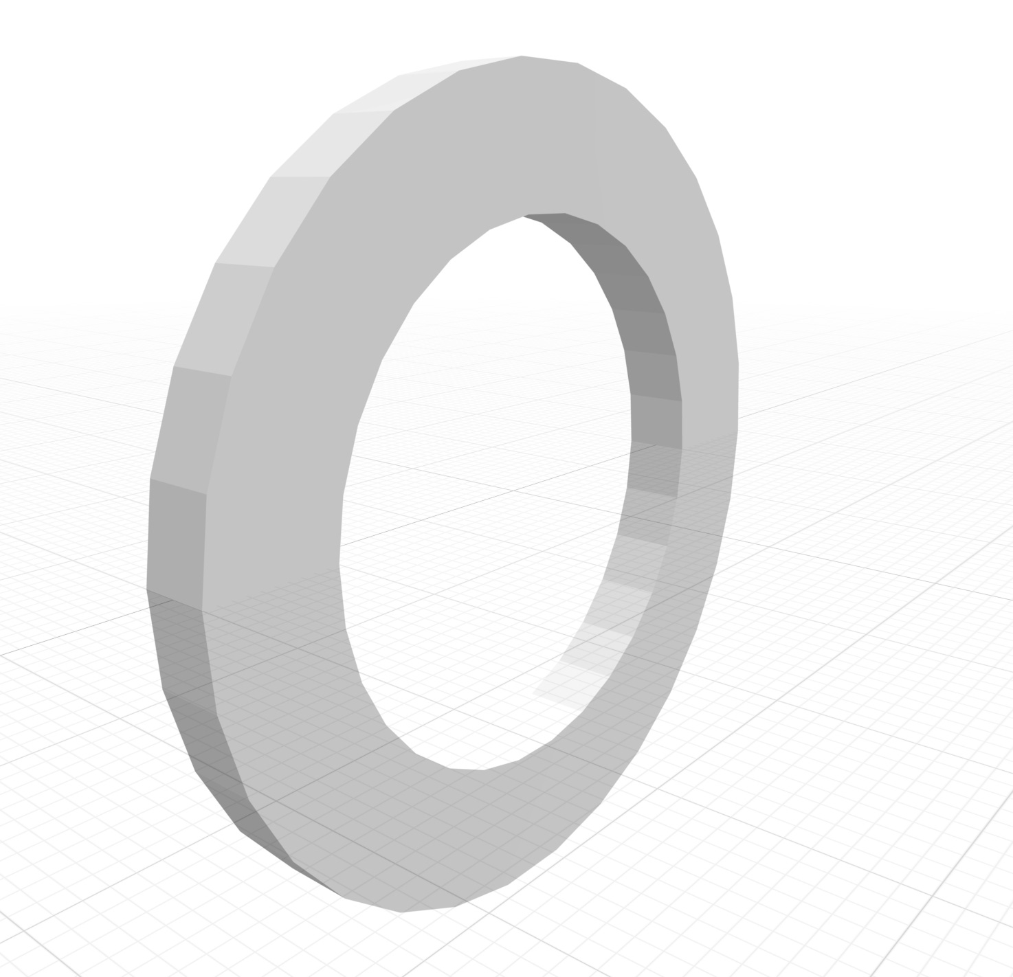
Transform Web (text-to-CAD software) was used to create the above geometry. The integrated LLM was used to calculate the stress in the washer given the loading conditions and generate python code to verify the calculation. The generated script produced an answer of 51kPa. The python script is shown below.
import math

def washer_stress(force_N, inner_d_mm, outer_d_mm):
    # Convert diameters from mm to meters
    inner_d_m = inner_d_mm / 1000
    outer_d_m = outer_d_mm / 1000

    # Calculate annular area
    area = (math.pi / 4) * (outer_d_m**2 - inner_d_m**2)

    # Calculate stress
    stress = force_N / area  # in Pascals (Pa)

    return stress

# Updated parameters
force = 20      # N
inner_d = 20    # mm
outer_d = 30    # mm

stress_pa = washer_stress(force, inner_d, outer_d)
print(f"Stress on the washer: {stress_pa:.2f} Pa")
The same geometry and loading condition was then run through a state-of-the-art, open source FEM software called deal.II. The max von Mises stress calculated by the software was 52.8kPa after 227 iterations over a mesh size of 1024 linear, hexahedral elements. Something to keep in mind is that stress is derived from strain/deformation using the finite element method, meaning that the governing equation actually contains a strain tensor and the stress is calculated in post-processing. This is why the material properties need to be given to run the software, because deformation depends on the Young’s modulus and Poisson’s ratio of the material. The stress distribution is shown below.
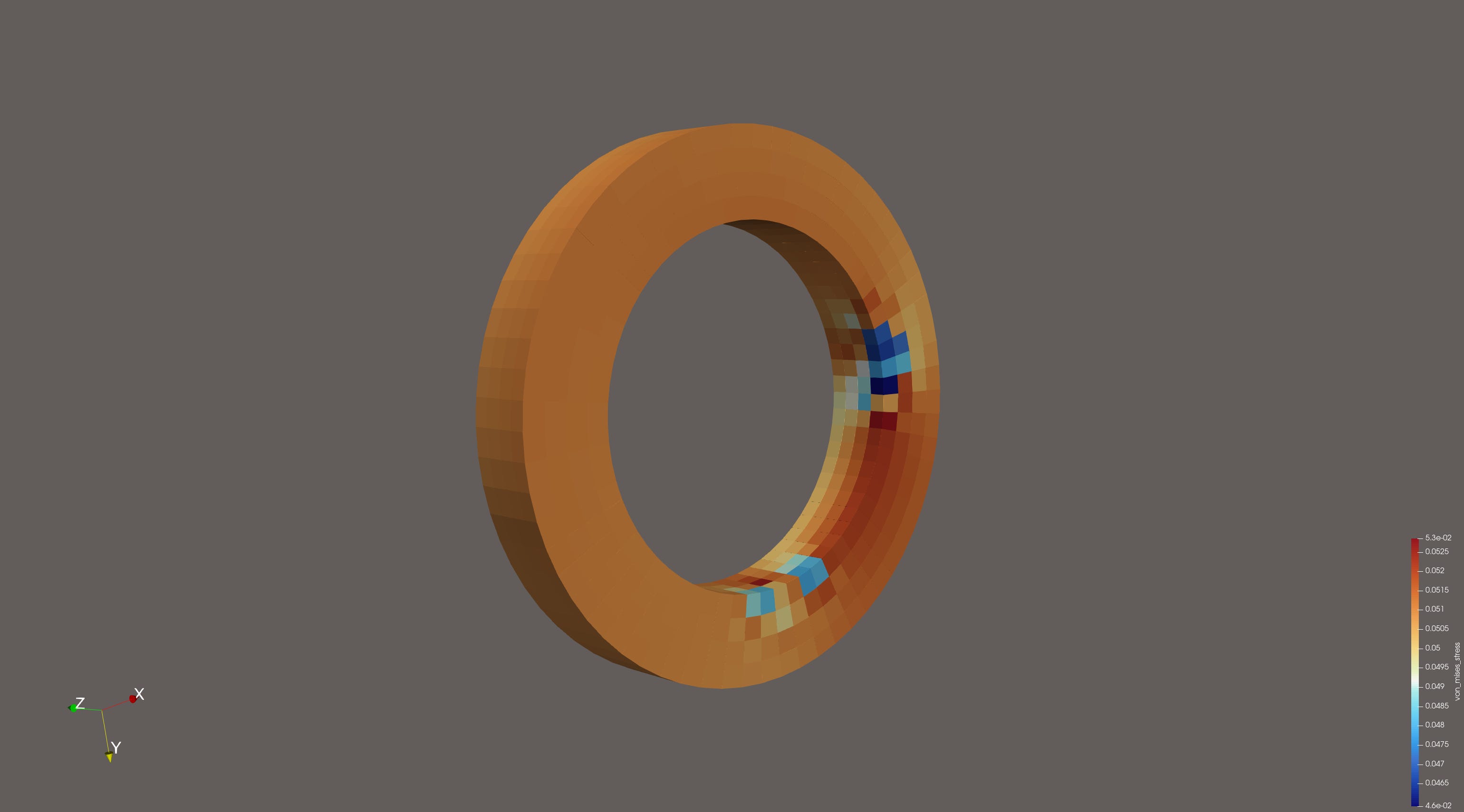
There is some variation in the stress distribution above. Some of this is probably due to user error in setting up the boundary conditions, but the sharp corners also add stress concentrations, which should see higher stress with enough cells in the mesh. Dark blue appears to be around 46.5kPa, which is only a 8.8% difference from the theoretical solution of 51kPa. The average looks like about 51.5kPa, which is also close to the theoretical solution.
Even though the BCs may be producing a slight asymmetry, the stress aligns with the theoretical behavior and should be suitable for a computational comparison.
Performance Comparison
The number of flops (floating point operations) can be used to estimate the computational or energy requirements of the simulation. This is calculated by summing the number of arithmetic operations the computer is required to perform on floating point numbers.
The python script generated by the LLM is 8 flops. The FEM software used 1024 mesh cells over 227 iterations with 4800 degrees of freedom. An LLM was used to produce code that would count the flops during the mesh generation, solution, and post-processing phases. The printout is shown below.
-------- FLOATING POINT OPERATIONS SUMMARY --------
Assembly phase: 85868553.00 FLOPs
Solver phase:   138614592.00 FLOPs
Stress calc:    369669.00 FLOPs
----------------
TOTAL:          224852814.00 FLOPs
                2.249e+08 FLOPs
--------------------------------------------------
To get a theoretical estimate of the flops to compare with, the stiffness matrix was printed out to see how sparse the matrix is. The sparsity of the matrix determines how many operations are performed during the solver phase, because only nnz’s (non-zeros) are included in the number of flops. The matrix is 4800x4800 with 292,032 nnz’s (non-zeros). This comes to about 1.27% filled, which is about 61 nnz’s per row. Each iteration performs about 2 flops per nnz for conjugate gradient method, so 2 * 292,032 is 584,064 flops per iteration. At 227 iterations, that’s about 133 million flops, theoretically. This lines up pretty well with the observed 139 million flops for the solver phase.
Compared to 8 flops from the python script, that is a huge difference. However, the LLM used flops to generate the python code also. Referencing GPT-3.5, which has 175B parameters, and assuming a typical response is about 100 tokens, the number of inference flops can be estimated as 2N flops per token. This comes to 35E12 flops per response.
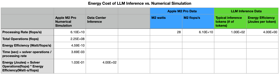
In fact, inferencing the LLM actually uses much more energy than the finite element analysis, as shown above. The energy estimate in the numerical simulation above was obtained by multiplying the total flops by the energy efficiency of a typical Apple M2 Pro. The inference energy cost was estimated using 4 Joules per token and 100 tokens per inference.
Even though the analytical model is less energy efficient when including the LLM inference, it saves engineering hours setting up an FE analysis, doing convergence studies, and interpreting results; all of which could take anywhere from half a day to over a week of engineering time.
The LLM only had to generate the constitutive relation once, and now that it is generated, the python code can be changed to account for scalar changes in the geometry or BCs. If the engineer wanted to reduce the stress in the part, he could simply increase the OD in the python code and rerun the code to get the stress. As long as he doesn’t change the geometry into a completely different shape like a square cross sectional area, or change the direction of the loading condition, the constitutive relation remains the same. With the FEM software, the engineer would have to regenerate the mesh and run the simulation again to find out what the new stress was.
This is a fairly simple example, but it could extend to more complicated geometries like pressure vessels, simple heat transfer models, beam deflections, or vibrations, where some of the differential equations are analytically solvable.
Conclusion
Analytical modeling cannot replace numerical models and simulations because most of the governing equations in nature are unsolvable. It may not be useful in cases where the geometries or BCs are changing by non-scalar values frequently, as this requires re-deriving the governing equations. It would also not be useful where the governing equations are typically nonlinear (unsolvable) like fluid flow, complex geometry, or non-homogeneous or anisotropic material properties. It could be useful in niche use cases with simple geometries and loading conditions to help engineers run quick calculations locally. Future engineers could run context-aware software that models the geometry and boundary conditions during the design process, determines if the governing equations are analytically solvable, and outputs and runs hyper-efficient, O(1) algorithms locally to provide the engineer with context while he designs.